IDAES-GTEP Tutorial Notebook

This notebook presents an introductory tutorial to using the IDAES-GTEP tool. To illustrate how to solve an expansion planning model, we use the PJM 5-bus test case with a few different assumptions on the network. With the solution of this model, this tutorial demonstrates some basic result visualizations on the investment options and grid operations. This tutorial describes how to create, set up, and solve the IDAES-GTEP expansion planning class ExpansionPlanningModel using a configuration with time period subsets.

Create Model with Time Subsets

The expansion planning model ExpansionPlanningModel in IDAES-GTEP with time period subsets requires the following parameters:

• stages: integer number of investment periods

• formulation: type of optimal power flow (OPF) problem when using EGRET. Currently, this model supports DCOPF and copper plate formulations. Note that this argument is not needed when not using EGRET.

• data: full set of model data.

• num_reps: integer number of representative periods per investment period.

• len_reps: integer length of each representative period in hours.

• num_commit: integer number of commitment periods per representative period.

• num_dispatch: integer number of dispatch periods per commitment period.

Once we define the parameters, we start building the expansion planning model. We start by importing the necessary libraries from Pyomo and IDAES-GTEP:

# Import Pyomo components
import pyomo.environ as pyo

# Import expansion planning components from IDAES-GTEP
from gtep.gtep_model import ExpansionPlanningModel
from gtep.gtep_data import ExpansionPlanningData

import pandas as pd

WARNING: DEPRECATED: Declaring class 'BaseRelaxationData' derived from
'_BlockData'.  The class '_BlockData' has been renamed to 'BlockData'.
(deprecated in 6.7.2) (called from
C:\Users\AppData\Local\anaconda3\envs\py311-black\Lib\site-
packages\coramin\relaxations\relaxations_base.py:43)
WARNING: DEPRECATED: pyomo.core.expr.current is deprecated.  Please import
expression symbols from pyomo.core.expr  (deprecated in 6.6.2) (called from
C:\Users\AppData\Local\anaconda3\envs\py311-black\Lib\site-
packages\coramin\domain_reduction\filters.py:4)
Interactive Python mode detected; using default matplotlib backend for plotting.

Include the data for the PJM 5-bus case study and load it to Prescient. This loads a default set of representative days.

data_path = "./data/5bus"
data_object = ExpansionPlanningData()
data_object.load_prescient(data_path)

C:\Users\AppData\Local\anaconda3\envs\py311-black\Lib\site-packages\egret\parsers\rts_gmlc\parser.py:254: FutureWarning: Support for nested sequences for 'parse_dates' in pd.read_csv is deprecated. Combine the desired columns with pd.to_datetime after parsing instead.
  df = pd.read_csv(file_name,
C:\Users\AppData\Local\anaconda3\envs\py311-black\Lib\site-packages\egret\parsers\rts_gmlc\parser.py:254: FutureWarning: Support for nested sequences for 'parse_dates' in pd.read_csv is deprecated. Combine the desired columns with pd.to_datetime after parsing instead.
  df = pd.read_csv(file_name,
C:\Users\AppData\Local\anaconda3\envs\py311-black\Lib\site-packages\egret\parsers\rts_gmlc\parser.py:254: FutureWarning: Support for nested sequences for 'parse_dates' in pd.read_csv is deprecated. Combine the desired columns with pd.to_datetime after parsing instead.
  df = pd.read_csv(file_name,
C:\Users\AppData\Local\anaconda3\envs\py311-black\Lib\site-packages\egret\parsers\rts_gmlc\parser.py:254: FutureWarning: Support for nested sequences for 'parse_dates' in pd.read_csv is deprecated. Combine the desired columns with pd.to_datetime after parsing instead.
  df = pd.read_csv(file_name,

Warning: The file './data/5bus/storage.csv' does not exist. Skipping loading storage data.

Build the expansion planning object ExpansionPlanningModel with no specific OPF formulation. DCOPF is built into the model, so it is the default OPF formulation.

mod_object = ExpansionPlanningModel(
    stages=2,
    data=data_object,
    num_reps=2,
    len_reps=1,
    num_commit=6,
    num_dispatch=4,
)

Create the GTEP model by calling the create_model method.

mod_object.create_model()

[    0.00] Creating GTEP Model
b.year = 2025
Cost data was not provided in m.mc instance (check DataProcessing for more details). Setting costs parameters to random values for now.
b.year = 2030
Cost data was not provided in m.mc instance (check DataProcessing for more details). Setting costs parameters to random values for now.

Apply transformations to convert the GDP problem into a Mixed-Integer Linear Programming (MILP) problem. To do this, first we apply the bound_pretransformation from pyomo.gdp to define lower and upper bounds that can be used in the Big-M transformation.

pyo.TransformationFactory("gdp.bound_pretransformation").apply_to(mod_object.model)
pyo.TransformationFactory("gdp.bigm").apply_to(mod_object.model)

Declare the solver and solve the problem.

opt = pyo.SolverFactory('highs')
mod_object.results = opt.solve(mod_object.model, tee=True)

Running HiGHS 1.11.0 (git hash: 364c83a): Copyright (c) 2025 HiGHS under MIT licence terms
MIP  has 24022 rows; 8476 cols; 71830 nonzeros; 4016 integer variables (4012 binary)
Coefficient ranges:
  Matrix [3e-02, 3e+05]
  Cost   [1e+00, 1e+05]
  Bound  [1e+00, 1e+03]
  RHS    [1e+00, 3e+05]
Presolving model
15528 rows, 4470 cols, 47568 nonzeros  0s
10828 rows, 3848 cols, 33464 nonzeros  0s
9928 rows, 2812 cols, 29492 nonzeros  0s

Solving MIP model with:
   9928 rows
   2812 cols (988 binary, 0 integer, 36 implied int., 1788 continuous, 0 domain fixed)
   29492 nonzeros

Src: B => Branching; C => Central rounding; F => Feasibility pump; J => Feasibility jump;
     H => Heuristic; L => Sub-MIP; P => Empty MIP; R => Randomized rounding; Z => ZI Round;
     I => Shifting; S => Solve LP; T => Evaluate node; U => Unbounded; X => User solution;
     z => Trivial zero; l => Trivial lower; u => Trivial upper; p => Trivial point

        Nodes      |    B&B Tree     |            Objective Bounds              |  Dynamic Constraints |       Work
Src  Proc. InQueue |  Leaves   Expl. | BestBound       BestSol              Gap |   Cuts   InLp Confl. | LpIters     Time

 J       0       0         0   0.00%   -inf            64682985.88726     Large        0      0      0         0     1.5s
 R       0       0         0   0.00%   53920107.88661  54828769.68073     1.66%        0      0      0      1497     1.9s
 L       0       0         0   0.00%   53920107.88661  53939831.82759     0.04%     2115    563      0      2231     5.7s
 L       0       0         0   0.00%   53920107.88661  53920107.88661     0.00%     2115    563      0      2905     6.4s
         1       0         1 100.00%   53920107.88661  53920107.88661     0.00%     2115    563      0      3023     6.4s

Solving report
  Status            Optimal
  Primal bound      53920107.8866
  Dual bound        53920107.8866
  Gap               0% (tolerance: 0.01%)
  P-D integral      0.109018724405
  Solution status   feasible
                    53920107.8866 (objective)
                    0 (bound viol.)
                    0 (int. viol.)
                    0 (row viol.)
  Timing            6.44 (total)
                    0.00 (presolve)
                    0.00 (solve)
                    0.00 (postsolve)
  Max sub-MIP depth 1
  Nodes             1
  Repair LPs        0 (0 feasible; 0 iterations)
  LP iterations     3023 (total)
                    0 (strong br.)
                    734 (separation)
                    792 (heuristics)

Process some results into dictionaries.

import pyomo.gdp as gdp

valid_names = ["Inst", "Oper", "Disa", "Ext", "Ret"]
renewable_investments = {}
dispatchable_investments = {}
load_shed = {}
for var in mod_object.model.component_objects(pyo.Var, descend_into=True):
    for index in var:
        if "Shed" in var.name:
            if pyo.value(var[index]) >= 0.001:
                load_shed[var.name + "." + str(index)] = pyo.value(var[index])
        for name in valid_names:
            if name in var.name:
                if pyo.value(var[index]) >= 0.001:
                    renewable_investments[var.name + "." + str(index)] = pyo.value(
                        var[index]
                    )
for var in mod_object.model.component_objects(gdp.Disjunct, descend_into=True):
    for index in var:
        for name in valid_names:
            if name in var.name:
                if pyo.value(var[index].indicator_var) == True:
                    dispatchable_investments[var.name + "." + str(index)] = pyo.value(
                        var[index].indicator_var
                    )

costs = {}
for exp in mod_object.model.component_data_objects(pyo.Expression, descend_into=True):
    if "Cost" in exp.name or "cost" in exp.name:
        costs[exp.name] = pyo.value(exp)

Generate some plots.

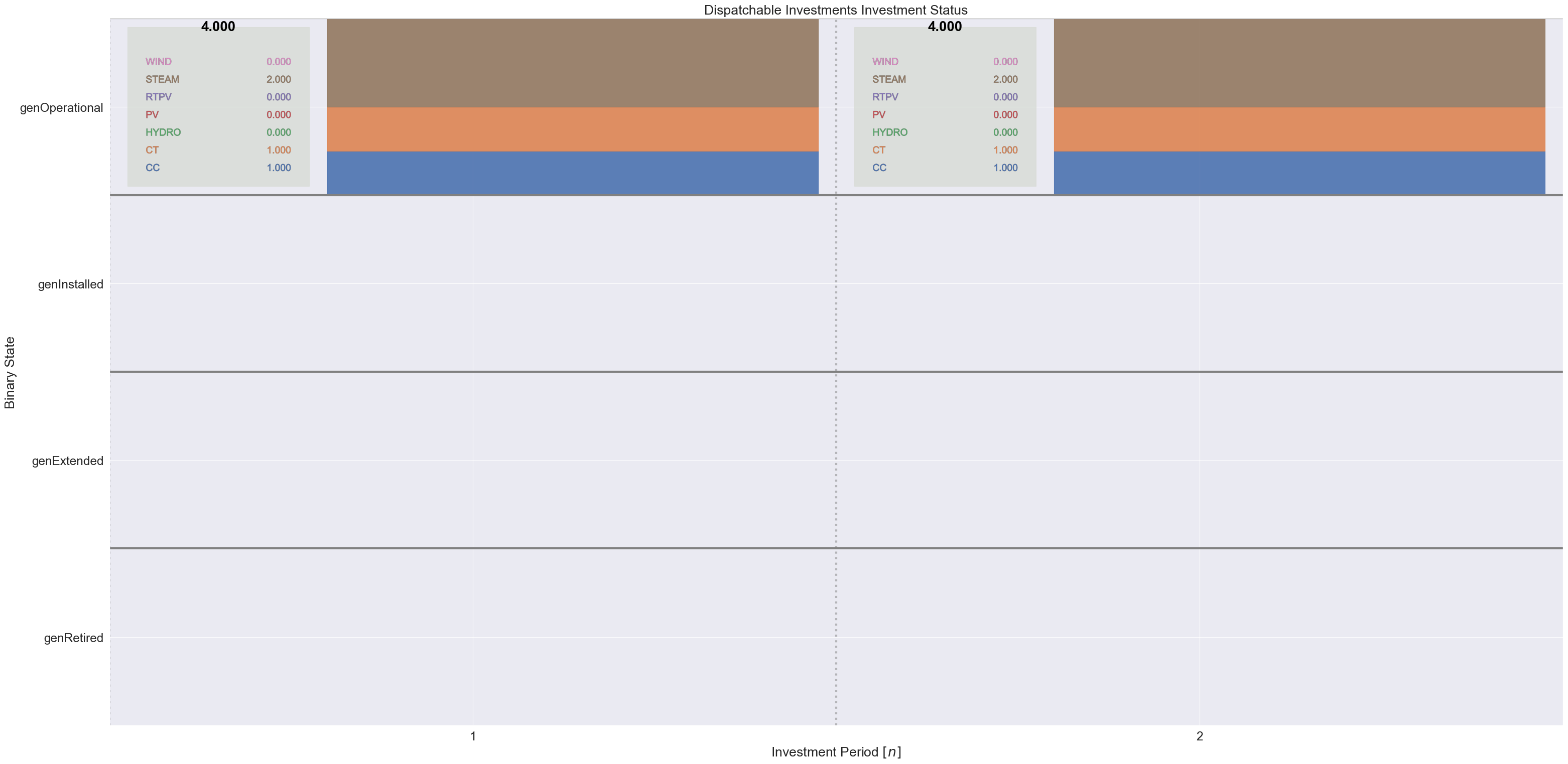
from gtep.tutorial_helper_fns import to_dict, plot_binaries

gens_pd = pd.read_csv("./data/5bus/gen.csv")
this_dict = to_dict(dispatchable_investments)
states_order = ["genRetired", "genExtended", "genInstalled", "genOperational"]
plot_binaries(this_dict, "Dispatchable Investments", states_order, gens_pd)
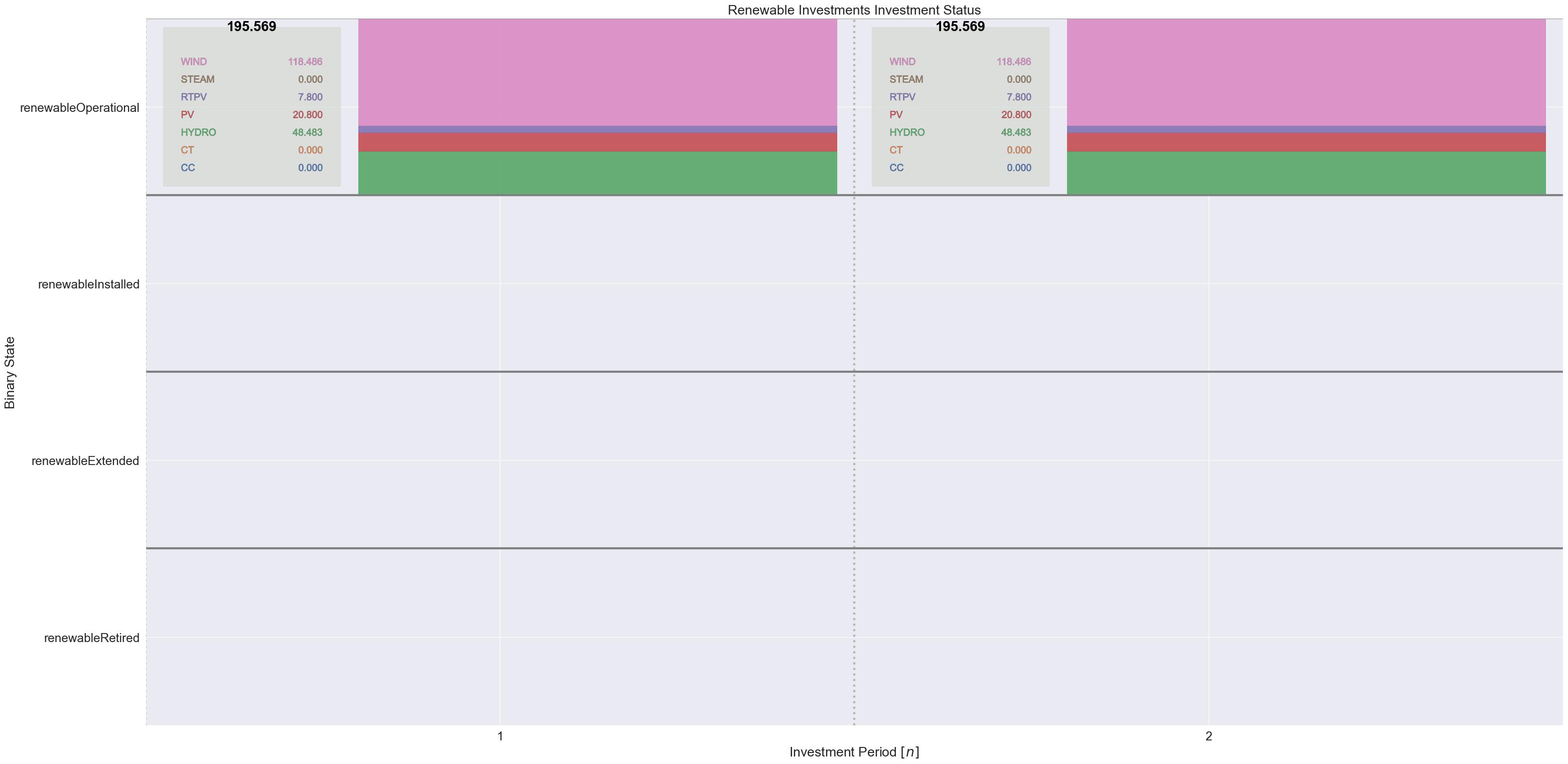
this_dict = to_dict(renewable_investments)
states_order = [
    "renewableRetired",
    "renewableExtended",
    "renewableInstalled",
    "renewableOperational",
]
plot_binaries(this_dict, "Renewable Investments", states_order, gens_pd)